Back in June came the exciting news of the first release of Crime Analysis in ArcGIS Pro 2.2. This is an extension for ArcGIS Pro and supports common workflows currently performed in ArcMap, along with new capabilities exclusive in ArcGIS Pro.
The extension is nicely organised into a single tab within the ArcGIS Pro Ribbon and bundles together current ArcGIS Pro tools with tools which are Crime Analysis originals. The Crime Analysis extension is available at no additional cost to customers with ArcGIS Pro, although some geoprocessing tools require a Spatial Analyst license. You can get the extension from ArcGIS Solutions.
I’ll focus on these exclusive tools and have used data from Greater Manchester Police to illustrate some. I’ve broken the list down into the same sections as the toolbar itself:
- Data Management
- Selection
- Tactical and Strategic Analysis
- Investigative Analysis
- Create and Share Information
Although being aimed at Crime Analysis, the tools will have applications in other areas and I’ll try and give a few examples along the way.
Data Management
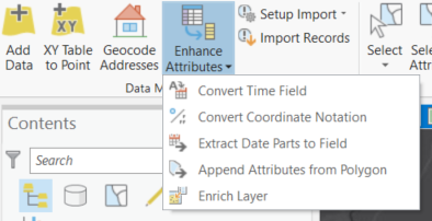
The first Crime Analysis original is the Extract Date Parts to Field tool. In short, it creates new fields containing date parts. For crime, this allows you to then select by time, day of the week or month and run analysis on specific dates.
You also have the Append Attributes from Polygon tool. Aptly-named, this tool appends fields from a polygon layer to points. For example, adding the precinct name to the crime point.
Away from crime where else would data management tools be needed? Looking at Boris Bikes in London perhaps? We could use the same tools to understand when and where Boris Bikes are most popular.
Selection
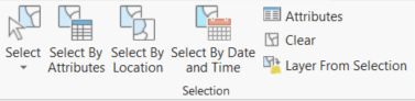
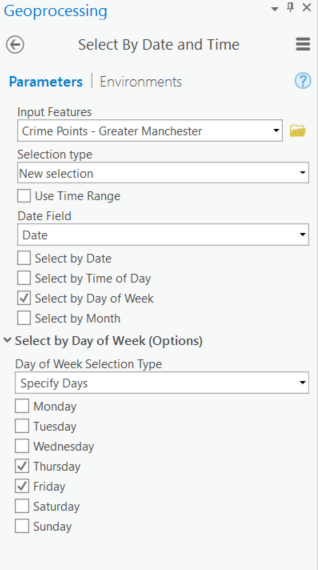
Select by Date and Time can select features based on date and time ranges (i.e. the last 30 days), or by parts (i.e. just Thursdays and Fridays). You could then use the Layer From Selection command to create a new layer based on your current selection and use this in your analysis.
Tactical and Strategic Analysis
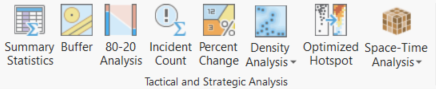
Tactical and Strategic Analysis focuses on analysing and understanding more long-term patterns within your data. The 80-20 Analysis tool calculates a cumulative percentage of incidents at locations. It supports the Pareto Principle, where approximately 80% of the effects (e.g. crimes) come from 20% of the causes (e.g. areas). The example below shows those clusters in the top 20% of reported crimes, highlighting key areas to target.
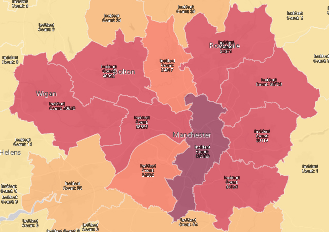
The next tool to show is Incident Count. This creates a new layer by aggregating points to polygons. In the example below, I have used Local Authority Districts to understand crime in the Manchester area. Labels are generated to show exact counts and, within the attribute table, a breakdown of the counts of each crime type for the local authority can be found. This can be extremely useful if you are focussing on a specific type of crime in your area.
We could also use the Incident Count tool in retail. We could aggregate supermarkets to local authorities and then break this down by a specific supermarket of your choice.
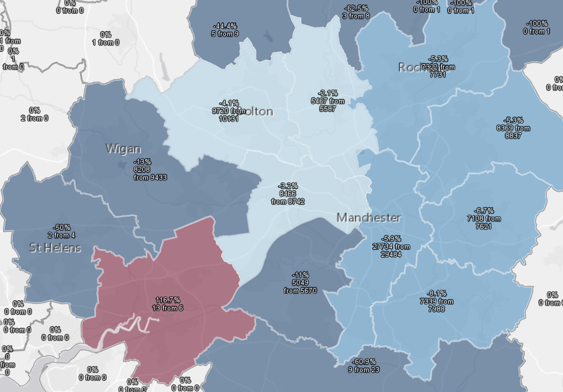
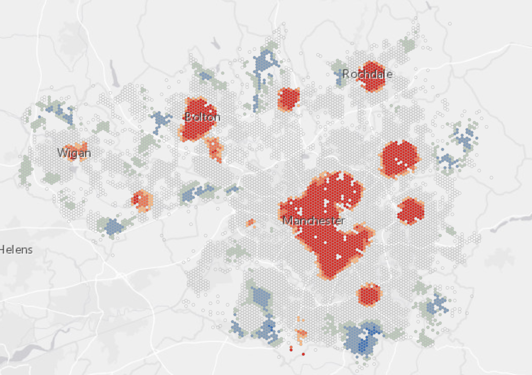
Percent Change calculates the percentage change in a polygon based on two input point layers of different time periods. Below, I compared crimes from the last three months of 2017 and the first 3 months of 2018. Areas in red have increased in crime, whilst areas in blue decreased.
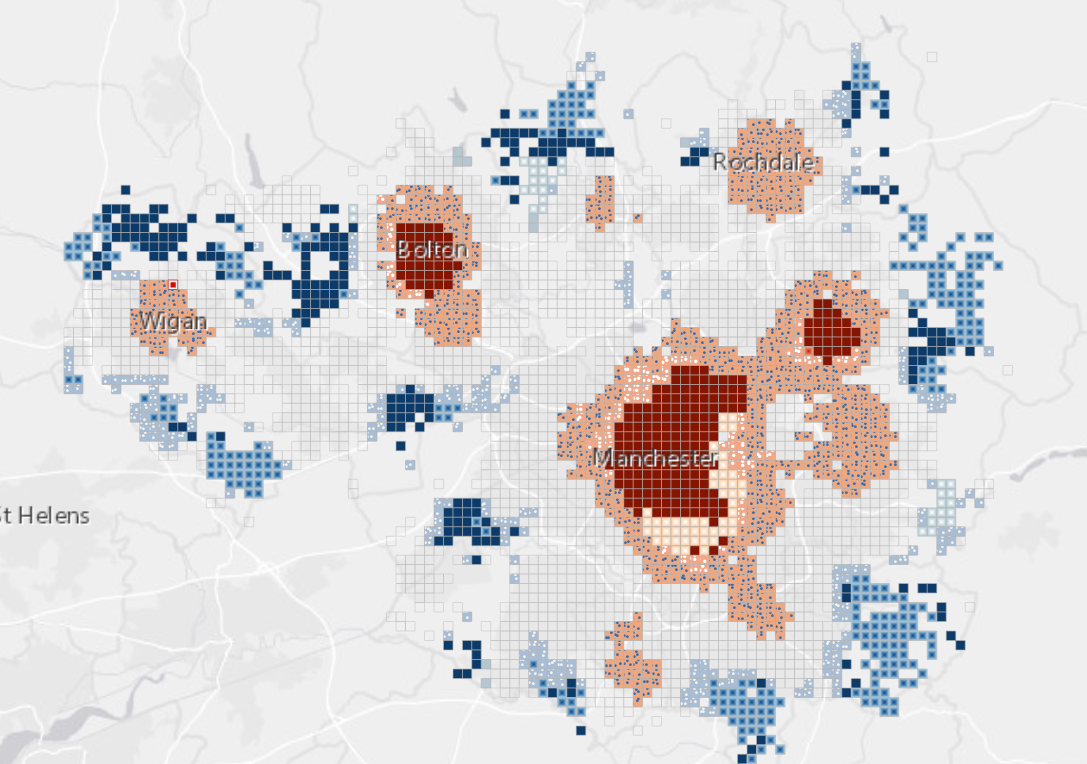
Density Change illustrates the change between two kernel density outputs from different time periods. Much like Percent Change, I calculated this for the last three months of 2017 and the first three months of 2018. Again, red indicates an increase in crime and blue a decrease.
These next two tools are not Crime Analysis exclusives but are important to be aware of. The Optimized Hotspot tool is fantastic for understanding statistically significant hot and cold spots using the Getis-Ord Gi* statistic.
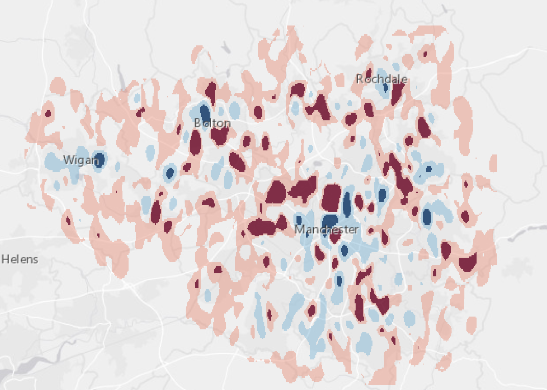
We can take this one step further by introducing time. Use the Emerging Hotspot tool by first creating a space-time cube. Emerging hotspots identify trends in the clustering of points through time and finds different hot and cold spot patterns. Use this help page for information on the various hot and cold spot definitions.
Compare the output below with the Optimized Hotspot one above. With the introduction of time, Manchester can now be divided into areas of persistent, sporadic, diminishing and oscillating crime. This analysis could also be useful when looking at road traffic accidents, habitat loss, or even natural disasters.
Investigative Analysis
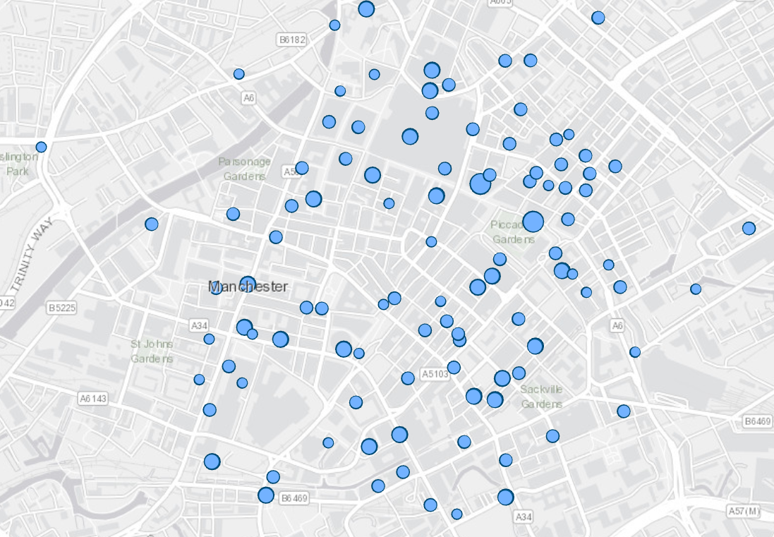
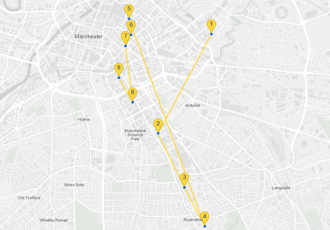
These tools focus on assisting investigations by looking at the relationships between different points. The Incident Sequence tool creates lines between related incidents based on the date field of those points, with the output showing the order they occurred. Here we have a string of bicycle thefts in Manchester over a 24-hour period.
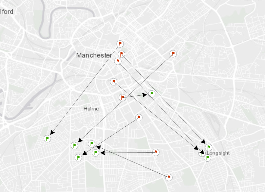
The Incident Path tool creates linking lines between two layers based on unique identifiers. This could investigate one-to-one relationships or one-to-many relationships such as gang member addresses to gang turf. My example looks at the same bicycle thefts (red flags) and then where the bikes were recovered (green flags). Outside of crime, this analysis could be useful to look at patterns of where locals live in relation to where they shop.
Create and Share Information
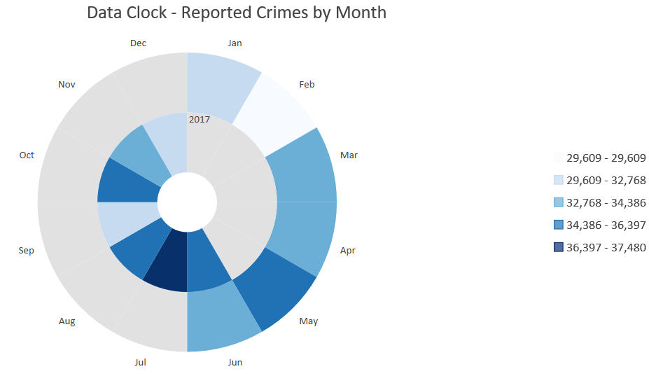
Whilst the options in this section aren’t exclusive to Crime Analysis, I still wanted to highlight one new addition. In ArcGIS Pro 2.2, the data clock chart was introduced – providing another great way to visualise your temporal data.
There we have it. I hope this blog has inspired you to try the new Crime Analysis tools on offer in ArcGIS Pro – whether you are a Crime Analyst or otherwise.
![]()