In today’s world, more and more organisations are starting to use Big Data techniques to analyse their data, which is increasing in volume and velocity every day. Cloud providers are both meeting and fuelling demand for these capabilities by providing powerful, elastic parallel processing services such as managed Spark environments.
But many of these services turn out to be incredibly challenging to use for Geospatial data. What we consider “normal” data in the GIS world rapidly becomes Big Data in these new processing environments, because many of them don’t support the concept of a Spatial Index. See for example this superb blog by the Ordnance Survey, Microsoft and Databricks which outlines some of the challenges and potential solutions.
Spatial Indexes are the petrol that makes GIS engines run. A spatial index can make a location-based query 100s or 1000s of times faster, in just the same way as a normal database index does with other types of data. Organisations such as Esri, Oracle, IBM, Microsoft and others have spent decades researching and implementing them. Within ArcGIS, if you display or query data in a File Geodatabase you are using Esri’s spatial index implementation. If your data is in Oracle, SQL Server, Postgres or SAP Hana, then typically ArcGIS will use that data store’s native spatial index rather than its own, making spatial queries as rapid (or almost as rapid) as attribute queries.
I believe that until these new Big Data environments increase their support for indexing geospatial data, many data scientists would be better off using Small Data techniques to do their large geospatial operations. I am going to show you a couple of examples to demonstrate how easy and quick this can be.
Challenge one
I will start with Ordnance Survey’s Open UPRN data. I have it in Parquet format, a common and efficient format for storing data for Big Data analysis. ArcGIS Pro 2.9 can read Parquet natively, but only some of its analysis tools understand it. Therefore, I will load it into a File Geodatabase to allow me to use any of the tools.
It takes a few seconds to copy the 1GB from Azure Blob storage, and then just under 10 minutes to load into a File Geodatabase using ArcGIS Pro running in Azure. The machine spec is a Standard NV16as v4 with P20 SSD disks (the default disks for this machine). The process of loading this data automatically creates the spatial index at the same time.
Actually spatial indexing of points is pretty easy. Even databases that have no spatial understanding of data will do a reasonable job of indexing points. So I also have 270,000 Land Register title extents from HM Land Registry’s National Polygon Dataset in good old Shapefile format.
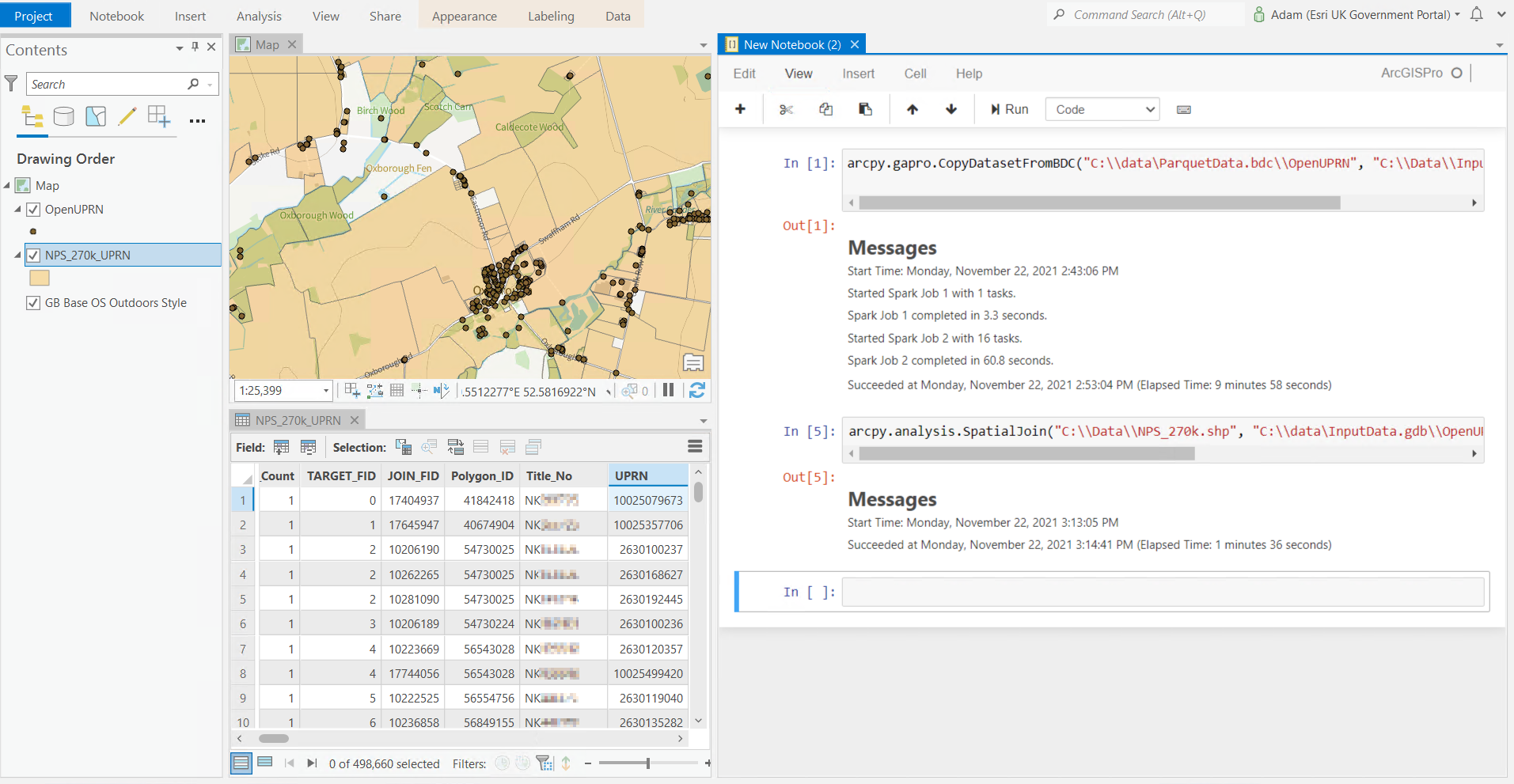
HMLR supplies a lookup table for UPRN against the title extent polygons, but I want to check this lookup table; I want to do my own assignment of each polygon to one or more UPRNs, based on which of the 40 million UPRNs sit geographically in each of the 270,000 polygons. Some polygons won’t have a UPRN, so no record should appear in the output. Some polygons will have multiple UPRNs, resulting in multiple records in the output. I want to do a Spatial Join between the 270,000 polygons and the 40 million UPRN points. I also want to write the results out to disk again so I can do follow-on processing.
Is this a Big Data operation? Only if you don’t use a spatial index! Using my Small Data techniques, generating a new polygon for each matching UPRN takes 1 minute 36 seconds to generate and write out to disk the 500,000 result records. You can see from my screenshot I am using ArcGIS Pro’s built-in Notebook environment to keep track of what I am doing.
OK that is quick. Let’s try more input polygons. I can’t make my Shapefile any bigger as they have a 2GB limit, so I’ll use a File Geodatabase to hold the input dataset. A spatial join of 1 million NPD polygons, against 40 million points, including writing the 1.9 million results to disk, took 5 minutes 9 seconds. The same operation using the 3.6 million polygons in the London region took just over an hour – this wrote a whopping 54 million results to disk (all the flats and Leaseholds in London I assume). Each result record contains about 50 attributes, so the results are many GB of data.
And I don’t have to worry about spatial indexes. ArcGIS ensures the indexes are kept up-to-date and used appropriately. And my datasets aren’t even in the same coordinate system! The Open UPRN data was actually loaded in WGS84 projection whilst all my existing NPD data is in British National Grid.
There are faster ways to do this processing in ArcGIS Pro – for example the Pairwise tools use parallel processing to do the actual work faster. There is also something else interesting. If you look carefully at my screenshot, you will see that some of the messages from the first step, CopyDataFromBDC (big data connection) refer to Spark. What is this?
ArcGIS Pro includes an entire Spark environment! This allows a subset of ArcGIS Pro’s geoprocessing tool library to chop problems up into discrete chunks that can be run in a highly parallelised way, perhaps more effectively than the normal Pairwise tools. And, unlike many of the Big Data environments I referred to at the start – where data scientists battle to process relatively small amounts of spatial data – ArcGIS Pro’s Spark environment comes with spatial indexing built-in.
Let’s try the whole NPD polygon dataset. A Spark-based Spatial Join between 30 million polygons and 40 million points. This manages to do the query and write 140 million output records to a File Geodatabase in just 103 minutes, most of which is the disk writes (remember each result record contains a polygon and 50 attributes). This is really a demonstration of the power of spatial indexes in general, not a particular feature of ArcGIS. I tried it natively in Postgres’s spatial extension PostGIS. Doing the same 30 million polygons against 40 million points, including writing the output to disk as a new table, took about 138 minutes for me. Note both datasets need to be in the same coordinate system in PostGIS.
OK points are pretty simple, but what about Polygon in Polygon? This is where things really get hard if you don’t use well-implemented spatial indexes.
Challenge two
Let’s try another real-world scenario. Fertilizer runoff from farms into rivers is a major concern for the Environment Agency, who conducts consultation and communication with the farming industry on the subject. In my hypothetical example, I am going to work out who owns every field within 500m of a river in England. This will allow me to write to the owners, to inform them for example of initiatives and grants, and to remind them of their obligations. In my letter, I want to include the river name if there is one as well as the grid reference of the identified field.
The Rural Payments Agency have an open dataset of Field Boundaries in England. In the dataset there are about 2.6 million records. I will use the Open Rivers dataset from Ordnance Survey, and for ownership information, I will use Esri UK’s TitleInfo data product. This product is just the HMLR National Polygon Dataset used in the previous test, enriched with some ownership information.
There are lots of different ways to do this analysis. Based on my Point-in-Polygon example, I’m not convinced either my business problem or my infrastructure justifies using ArcGIS Pro’s Spark-powered tools, so I will use the Pairwise tools instead. As I am doing multi-step processing, I am going to write intermediate datasets to ArcGIS Pro’s memory workspace to avoid overhead from the disk writes.
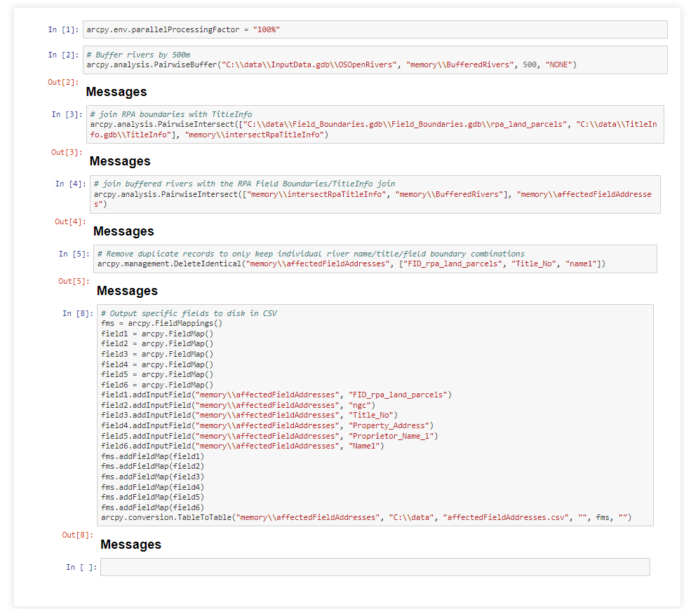
Here is the process I used:
- Buffer the Ordnance Survey Rivers dataset by 500m. This generates 186,000 polygons in just 12 seconds.
- Use the Pairwise Intersect tool to join the 2.6 million English field boundaries with the 30 million England and Wales TitleInfo records, to generate a dataset containing the ownership information of each Field. This generates 4.4 million records in 22 minutes.
- Join these 4.4 million records with the 186,000 buffered rivers to get in in-memory result table. This generates 6.9 million results in just over 8 minutes.
- Remove redundant records so there is only one record per Title per Field per River, because this is what I will use for my hypothetical mailshot. I am anticipating each proprietor receiving a list of the identified fields, river names and grid references. This leaves 3.7 million remaining records and executes in 10 minutes 46 seconds (maybe I should have indexed the fields!).
- Export just the fields of interest (RPA field identifier, British National Grid reference, Land Registry Title Number, Property Address, Proprietor Name, Proprietor Address, River Name) into a CSV on disk for a mail merge operation outside of ArcGIS. This creates a 266MB CSV file with the 3.7 million records in 2 minutes.
Total processing time: 43 minutes.
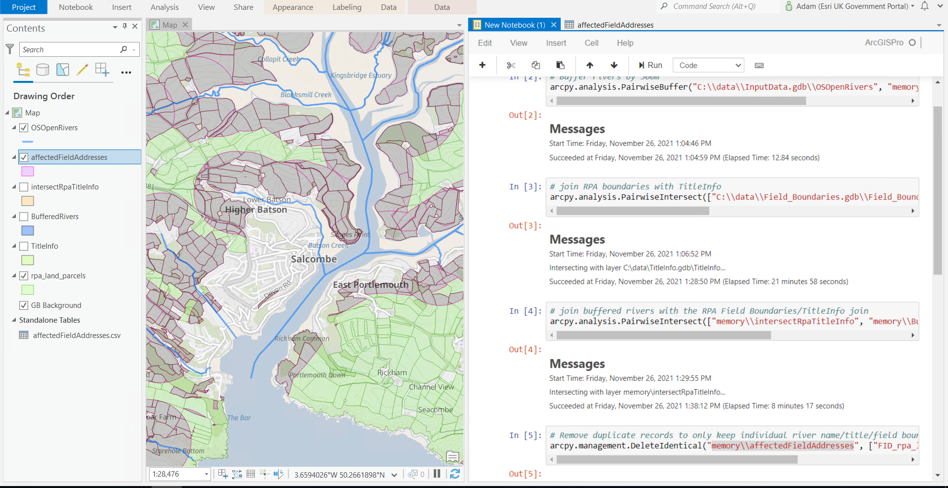
Here is the Notebook I used for this example:
So what?
Of course ArcGIS does much more than fast spatial joins. As well as visualisation, it includes a huge range of geoprocessing tools and complex topological operators, it can visualise hotspots and emerging patterns in both space and time, it understands connectivity and networks, and it can perform spatial analytics in real-time, streaming data of hundreds of events per second.
This investigation demonstrates to me that large geospatial problems, such as national analysis of detailed data, can be easily performed on modern technology. And working in this new world does not mean abandoning the decades of geospatial research and development in the industry. Instead, it can mean using existing geospatial data science tools such as ArcGIS in modern cloud computing platforms. If you have a little bit of knowledge of working with spatial data, I believe you can save huge amounts of money in your data science operations. This is in terms of both compute resources and in terms of people to drive it.
But I do understand moving between the different processing paradigms of old world and new might be tricky in many workflows and in many organisations. And sometimes, the best tool for the job is the tool you already know. For an organisation with no current ArcGIS capability or experience, there is a learning curve in doing the analysis I have done above. So I am very excited that Esri is soon releasing a set of new capabilities that bring our decades of spatial research and development all the way into the new world as well as the old – the ability to embed Esri capabilities directly in your native Spark environment. More on this in my next blog post. Watch this space!