Time series forecasting – what is it, why would I use it, and how can I get started? In this blog, I’ll be taking you through the ‘what, why, and how’ of time series forecasting with ArcGIS Pro and how it could add value to your decision-making. I’ll begin by giving a brief introduction to time series forecasting. Following that, I’ll cover some common mistakes that are made with gathering data and how to avoid them. Finally, I’ll end by introducing you to Esri’s time series forecasting toolset and a step-by-step tutorial for how you can start creating time series forecasts with a spatial focus for yourself – all without needing any previous experience with statistics!
The time series forecasting toolset is available for all ArcGIS Pro license types – Basic through to Advanced.
The Basics
A time series is a set of data points linked to a corresponding time (e.g. hour, day, month, year, etc.). Ideally, time series data contains data points that are collected at consistent intervals over a certain period of time, rather than just intermittently or randomly. This allows any time series analysis that’s carried out to more effectively identify trends within the collected data, and more accurately make estimates for how similar data points may present themselves in the future. Enter, time series forecasting.
Time series forecasting is a technique used for estimating future events by interpreting past trends with the assumption that future events will continue to follow similar patterns. This is done by building best-fit models which resemble the trends observed in historic time series data and using these to extrapolate future values. Time series forecasting isn’t an exact prediction of what’s to come. You could call it a best guess; and the more comprehensive time series data that’s fed into the model, the better the guess.
To help cement the concept of time series forecasting, we can take the example of a retailer. Each year, during the holidays, sales revenues tend to increase. During the off-season, the reverse is typically true. Though it’s easy to roughly estimate whether sales will rise or fall in one season compared with the last, it’s difficult to know by how much. If we have time series data of sales revenue for every day/week/month spanning several years into the past, time series forecasts can use this historic data to model upcoming sales volumes and repeating trends can be more finely identified.
Uses for Time Series Forecasting
Time series analysis can help organisations explain the underlying trends in their temporal data. Time series forecasting takes this a step further by using the temporal patterns within data (such as seasonality or cyclical behaviour) to predict likely future outcomes. Although, things don’t just happen in time, but also in space. So, visualising a time series forecast spatially can add even more clarity to the distribution of likely future events in both time and space. Knowing how future events may unfold in this way can help people make better pre-emptive decisions to maximise important standards such as safety, efficiency, and costs.
“In decisions that involve a factor of uncertainty about the future, time series models have been found to be among the most effective methods of forecasting.”
– Anais Dotis-Georgiou
Common real-world examples where time-series forecasting is used include:
- Forecasting customer traffic to optimise staff schedules
- Forecasting the demand of a product to optimise the storage of inventory
- Forecasting infection rates in different locations to optimise responses
It’s important to always remember that there are ultimately limitations when dealing with the future and the unknown. Time series forecasting isn’t a perfect technique for predicting future outcomes. Before beginning any time series forecast, spend some time considering whether it’s the best tool for your intended purpose. Depending on the available data and the type of forecast that’s being done, the outcomes and their reliability can vary. If you decide that it’s the right technique, there are steps you can take to increase the accuracy of your forecasts. That journey begins with considering your data.

Shipping Containers by Tom Fisk
Data Considerations
It’s important to check that the data you plan to use is fit to be forecast. Below, I’ve listed five common considerations that you can use against your data. As promised, I’ll do my best not to get statistics heavy.
1. Number of Observations
Time series forecasting relies heavily on the amount of data available. This concept of ‘more data equals better analysis’ holds true with any form of data analysis, and time series forecasting is no different. The more points of observation we have, the better our models will fit our data. It also allows predictive models to distinguish between trends and noise in the data. For example, does the data follow patterns of seasonality despite the occurrence of a few anomalies? This is harder to tell when the dataset used is small. So, the more data that is available to us, the more accurate our forecasts are likely to be – and vice versa.
2. Time Horizons
A time horizon is how far into the future you’re generating a forecast for. The further you attempt to go, the more unreliable your estimates will be. If your dataset contains a large amount of short-term data, you should avoid creating forecasts with long time horizons. However, in such cases, short-term forecasts still generate good approximations. Most forecasting tools will be able to display the confidence of predicted values at varying time horizons which you can use to assess any forecast that you generate.
3. Random Data
Random events will never be forecasted accurately. This is true no matter how much data we gather or how consistently we gather it. For example, the lottery numbers can be recorded every week, but you wouldn’t be able to predict the next winning numbers. The lottery is designed to be random; so, historic patterns will not reflect future ones and any similarities observed will be coincidental.
4. Data Quality
A standard requirement for any data analysis technique is the use of good quality data. Data that’s of poor quality can result in wildly inaccurate time series forecasts. Typical guidelines for data quality include making sure data is: not duplicated, in a valid format, collected consistently and collected at regular intervals.
Among these, it’s especially important for the time series data to have been collected at regular intervals for the period of time being analysed. Having a ‘complete set’ of data without gaps helps us to better spot trends. These can include cyclic patterns or seasonality effects which gaps in our data might hide. Fewer gaps also make it clearer whether an outlier is truly an outlier, or if it’s part of a larger pattern.
5. Stationarity
To conceptualise what’s meant by stationarity, imagine a frictionless pendulum. Yes, it swings back and forth, but its motion will always follow the exact same pattern. The same can be said for stationary data; it may change over time, but certain fundamental properties always stay the same. To build a time series model that can reliably estimate future values, the data we use has to be stationary.
Stationary data is defined by the following properties:
- Constant mean
- Constant variance
- Covariance is independent of time
There are tests you can run on your dataset to find out if it’s stationary or not, the Dickey-Fuller test being a common one. Transformations also exist that can convert your data from non-stationary to stationary while still retaining the properties necessary to carry out a time series forecast. You can learn more about stationary datasets, the Dickey-Fuller test, and transforming non-stationary datasets in an article written by ‘towards data science’.
Esri’s Time Series Forecasting Toolset
Now that we’ve covered what time series forecasting is, when you may wish to use it, and how to prepare your data, let’s take a look at what capabilities the Esri’s time series forecasting toolset has. There are four different forecasting tools depending on the type of data being forecasted and the type of output required by the user. The toolset is also designed to visualise the distribution of its forecasts spatially to assist informed spatial decision-making.
You can find documentation for each tool in Esri’s time series forecasting toolset here.
1. Curve Fit Forecast
Time series data comes in all shapes and sizes. Some might have a linear trend while others follow a more S-shaped curve. This toolset is designed to help you deal with that level of variety between time series data. If you don’t know the curve that best describes your study area, you can select ‘auto-detect’ and this tool will automatically suggest the most suitable statistical model that you can use for your forecasts.
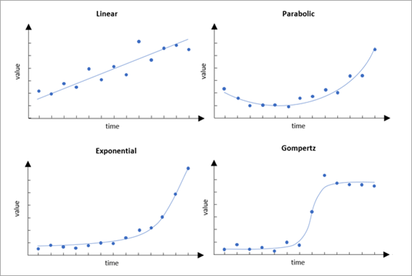
Four curve types are shown
2. Evaluate Forecasts by Location
While you can use a single model across your entire study area, you can also allow your models to vary across space. So, if you’ve broken your study area into smaller locations, in some locations this tool may choose a curve-fit forecast because the time series in those locations follow those common patterns. In others, it may choose what’s called a random forest-based approach because of the complexity of the time series there. This tool allows us to map different forecasting models across our study area depending on how well they fit in each location. So when we see different locations for which the same model applies, it gives us a valuable insight that those locations most likely also share similar characteristics.
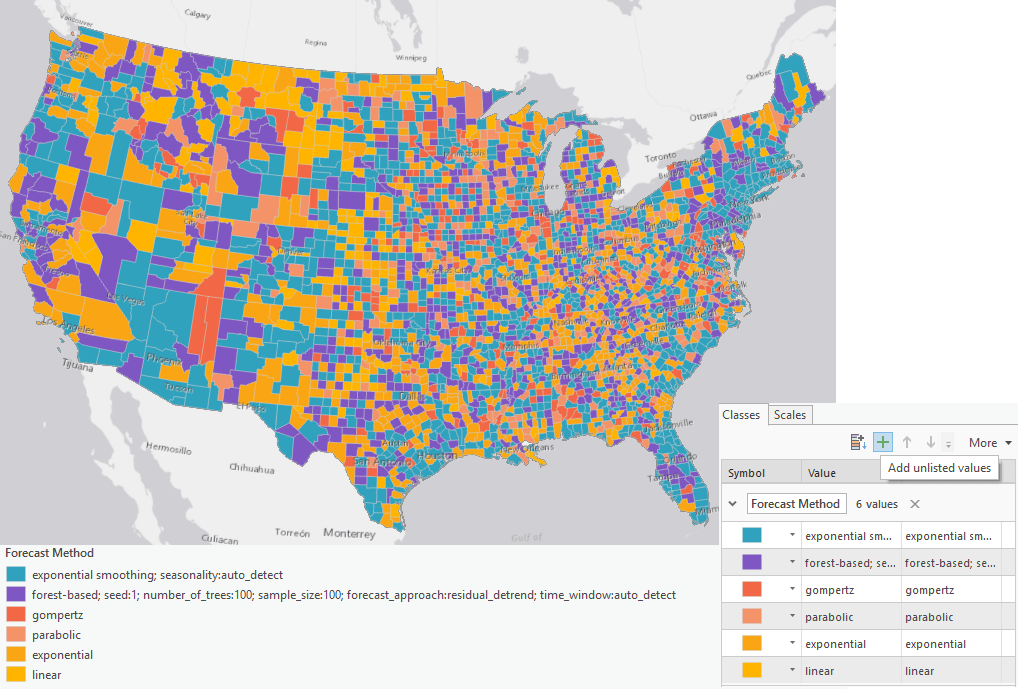
Evaluate Forecasts By Location output
3. & 4. Exponential Smoothing & Forest-based Forecasts
Both exponential smoothing and the random forest-based approach are good at dealing with complex time series, including seasonal or cyclical trends in our data which can be tricky when forecasting.
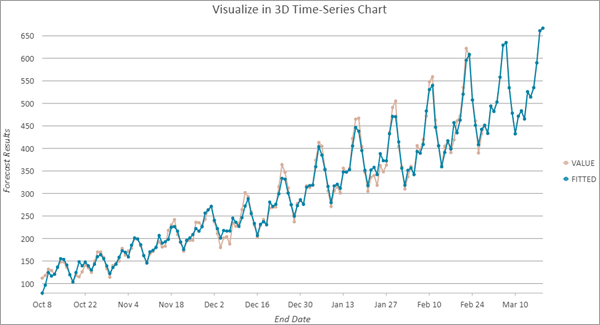
The graph shows a cyclical trend
Finally, one of the most important outputs of each of the tools is in the form of pop-ups. Within each pop-up, which is automatically generated, we can see our measured data in blue, our forecast in orange, and the uncertainty around that forecast. It gives us a valuable sense of how the model fits location by location across the study area. Pop-ups are available for every area that you’ve run a forecasting model for and can be viewed by clicking on the study area on your map.
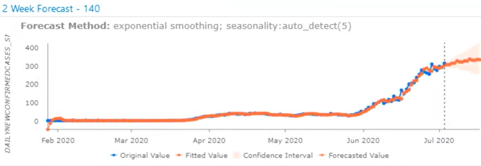
Forecast pop-up graph
Esri’s Time Series Forecasting Tutorials
The tutorials showcase different elements of the toolset by guiding you in carrying out your own epidemiological study, for monitoring and forecasting the spread of COVID-19 cases in the United States using open-source data. Monitor the current state of the virus, plot the rate at which it’s progressing, and forecast what may happen over the next two weeks. This tutorial will show you how the time series forecasting toolset helps us do just that. To have a go yourself, you can find all four parts of the tutorials here.
My takeaways from trying the tutorials:
When I first started learning about time series forecasting, I immediately went to these tutorials to see what I could pick up. They’re incredibly beginner-friendly because of how clearly the steps are laid out, and the fact that they’re broken up into four bite-sized chunks makes them even more so. I didn’t know the difference between the different forecasting models that exist, but, thankfully, the forecasting tools were able to automatically identify trends and suggest the most suitable statistical model for me to use.
No coding skills are necessary to complete the tutorials. You’ll find that running a Python script is one of the first steps used to clean up the original dataset. If you feel up to it, the code is provided for you to edit and run on ArcGIS Pro for yourself. Although if like me, you’d rather download the post-Python dataset directly from the Esri website, you have that option too!
Practice is the best teacher, even if it’s daunting. Following the tutorial step by step the purpose of certain tools and potential workflows begin to become clearer. Once you’ve completed the tutorials, feel free to have a go at running your own time series forecasts from other types of data.
Happy forecasting!