In the UK, the 10 hottest years on record have all been since 2002 and in the summer of 2022, July and August were the warmest ever. Despite periods of rainfall, hosepipe bans were put in place across large areas of the country.
As a result of these events, I wanted to investigate whether extreme weather is becoming more frequent in the UK, and which regions are experiencing the biggest change. Throughout this mapping process, I encountered many obstacles so I am going to take you through the journey on how I ended up with the final maps.
The Data
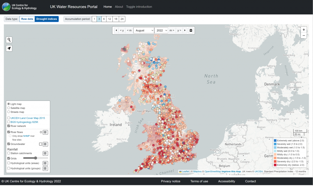
The data I used for this project was from the UK Centre for Ecology & Hydrology (UKCEH) Water Resources Portal. This portal contained a UK dataset showing the monthly Standardized Precipitation Index (SPI) going back to 1862. The SPI is an index of precipitation and shows “for a given location and month, how much the rainfall deviates from the long-term average” – i.e. how much the rainfall differs from the rainfall typically expected. This meant that I could compare different regions of the UK. UKCEH splits the UK into 117 “hydrological areas”, and the SPI values were provided monthly for each.
The Vision
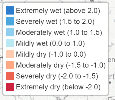
I now started to think about how to visualize this. Firstly, I categorized the SPI values into the precipitation categories provided by UKCEH such as Extremely Dry and Moderately Dry. Then, I created a choropleth map for each month between 1922 and 2022 (i.e. the last 100 years).
However, having individual monthly maps left me with no real clear story. This is where the ArcGIS Pro animation tools come in – I could create a short animation which iterated through each of the months. I envisioned that the animation would show Extremely/Severely Dry weather becoming more frequent over the century.
The animation
After spending a few days collating the data and trying out the animation tools, I created an animation showing the precipitation classification for each month for the past 100 years. However, I quickly realised this was not showing the story I wanted – I hoped to see the map ‘breathing’ with seasonal changes and the frequency of Extreme events becoming more common, but no clear conclusions could be drawn. Also, 100 years of data resulted in around 1,200 maps to animate through, so it was very fast and confusing.
After several attempts at slowing the animation down, I quickly decided that static maps would be a better option.
Static Maps
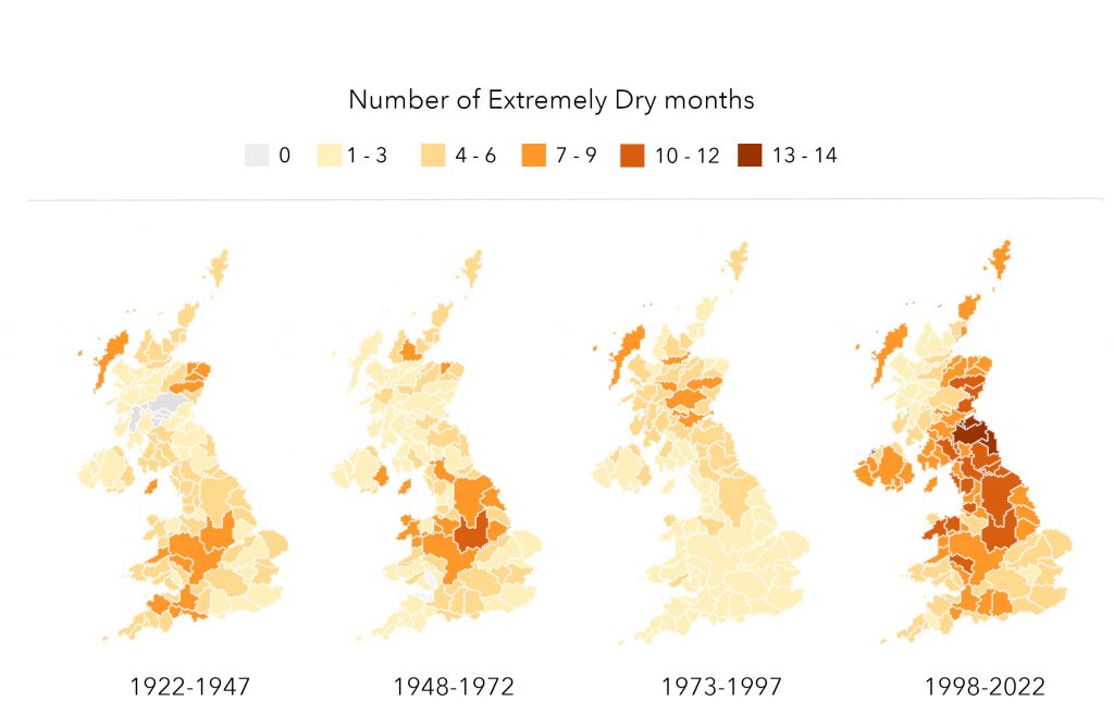
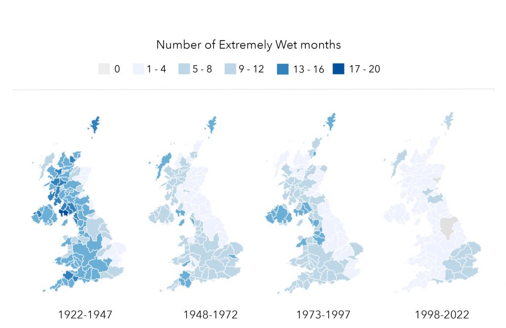
Feeling like I was back at square one, I had to think about the best way to display this vast amount of data on a static map. It seemed intuitive to break the 100 years down into chunks and I settled on 4 maps, each showing data for 25 year periods. Also, instead of looking at the whole range of precipitation categories, I thought it would be interesting to look at just extreme values – Extremely Dry and Extremely Wet. For each hydrological unit, I totalled the number of Extremely Dry months and Extremely Wet months for each 25 year period, creating 4 maps for each.
I also needed to consider colour, as the maps needed to show dry and wet weather. I avoided red tones, as this would give the impression of heat, and settled on a brown-yellow colour scheme for the Extremely Dry maps. For the Extremely Wet maps, a blue colour scheme was used.
My final maps are shown below:
Which areas had seen the most change?
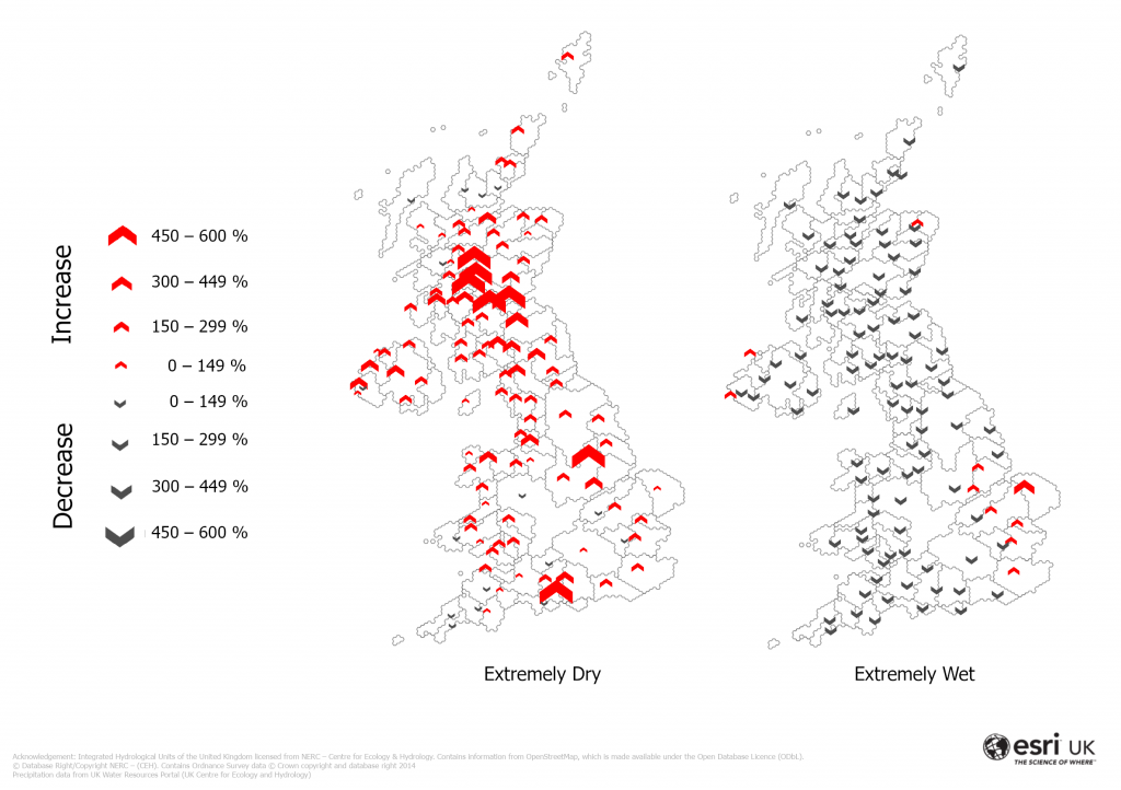
The static maps clearly showed that overall, Extremely Dry weather had increased and Extremely Wet weather had decreased between 1922 and 2022. However, I also wanted to investigate which areas had experienced the greatest change. I calculated the percentage change, comparing the total number of Extremely Dry months in the last 25 years (1998 – 2022) with the first 25-year time span (1922 – 1947) for each hydrological unit.
I first visualised this percentage change as a choropleth map but decided this was not the best approach, as these are usually used to display counts and amounts. The best symbology option would be proportional symbols – with the size of the arrow representing the extent of the change and orientation showing the direction of change. Through this visualization method, it was much easier to see which hydrological units had experienced the biggest increase/decrease in extreme weather over the last 100 years.
My final maps are very different to the maps I envisioned I would have been creating at the start of this journey. I had to make many cartographic decisions, as well as logistical decisions about the story I was trying to tell. Whilst the animation tools in ArcGIS Pro are extremely useful, they did not take the data in the direction I wanted it to. It was only by trialling out different options that I settled on a story and visualisation technique that I was happy with.
For more tips and tricks on how I created this map, you can check out the Map Gallery. There are also some useful blogs on creating animations through time in ArcGIS Pro, as well as how to make beautiful maps!
Happy Mapping!